
Background:
On September 26, 2016 the Cedar and Wapsipinicon rivers in Iowa experienced a torrent of water producing a flood wave that breached the riverbanks. The water level of the Cedar River measured ~20 feet — 8 feet above flood stage—near the city of Cedar Rapids. Palo, Iowa is a town upstream of Cedar Rapids and is comprised primarily of farmland, additionally they do not have a forecast location to give warning. I used rasters to create flood images and then applied thresholding, multiband Landsat imagery, and classification techniques to the images.
# Libraries
library(knitr)
library(units)
library(readxl)
library(sp)
library(raster)
library(tidyverse)
library(getlandsat)
library(sf)
library(mapview)
library(raster)
library(osmdata)
Color stretch:
When a color stretch is applied, the maximum and minimum colors in the images become the new range of colors. The result of the stretch is that the features being highlighted by the given RGB channel are more emphasized and clearly seen in the image.
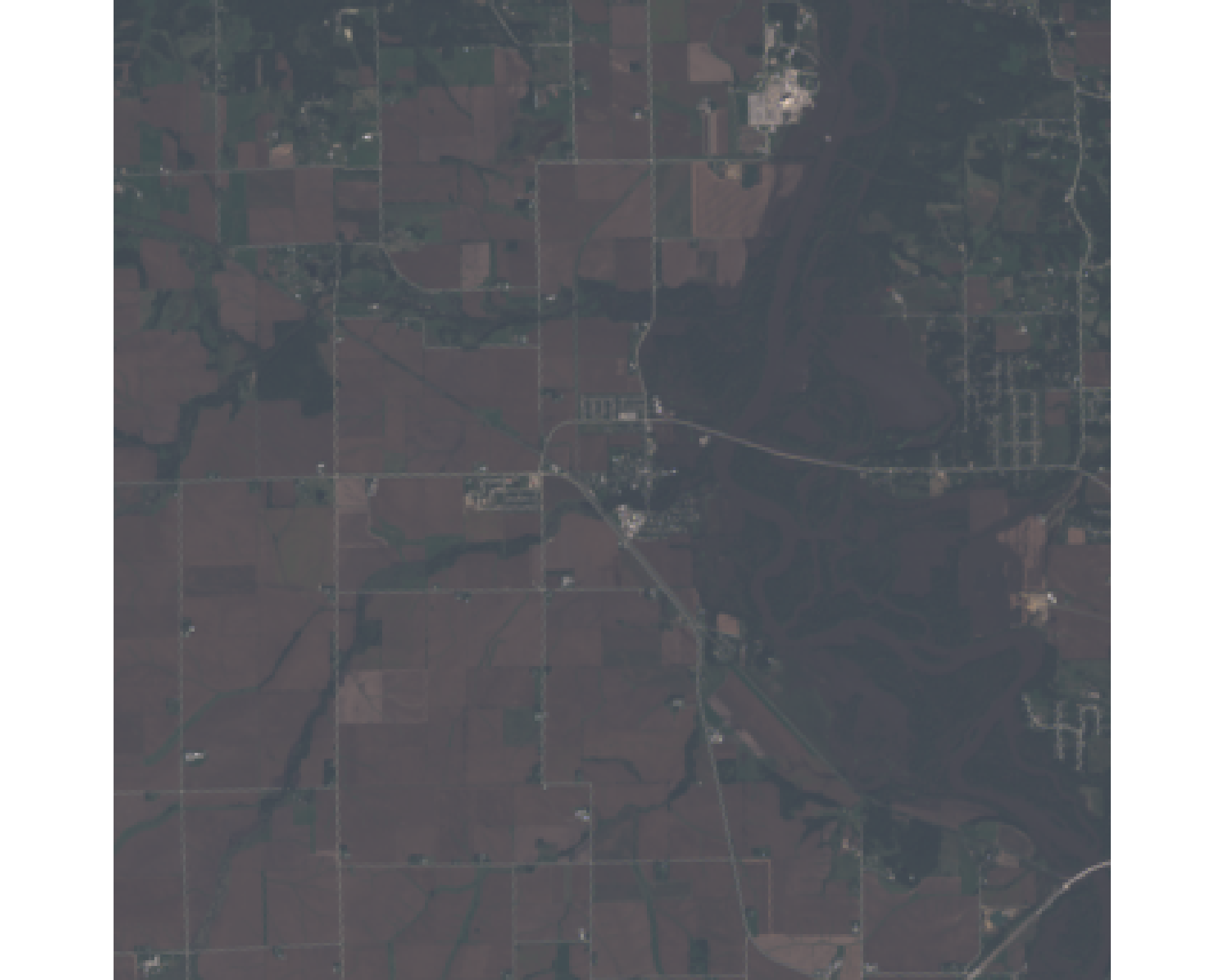
Figure 1: (4, 3, 2) Natural color . This is the closest true image bandwith. It is also prone to atmospheric interference
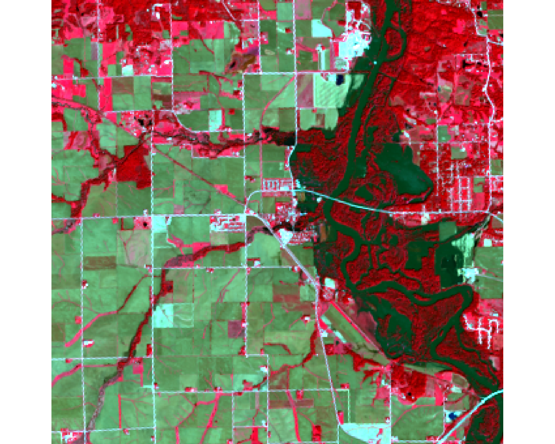
Figure 2: (5, 4, 3) Color infared with a lin color stretch. Color infared does a good job of differentiating different types of vegatation as well as the health of the vegetation.
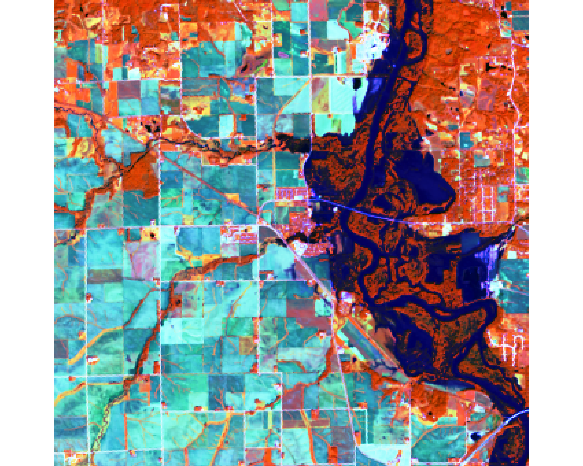
Figure 3: (5, 6, 4) False color with a histogram color stretch. False color is good at seperating water from land in an image.
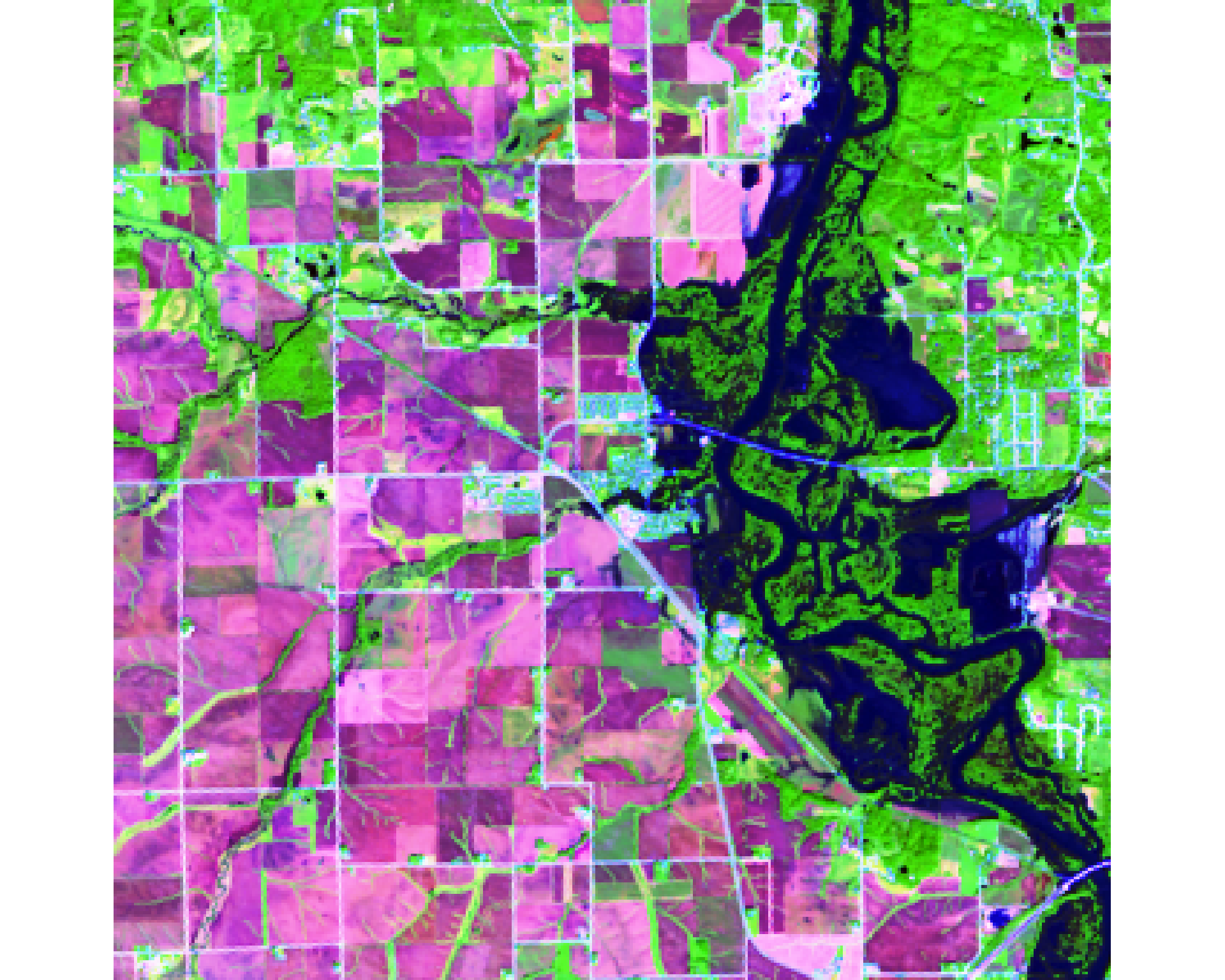
Figure 4: (6, 5, 2) False color for agriculture with a histogram color stretch. In this bandwith agricultural crops appear as a vibrant green, non-crop vegetation appears in a dull green, and bare earth appears in fuchsia.
# NVDI
x = (r$NIR - r$Red)/ (r$NIR + r$Red)

ndvi_func = function(x) {
  ifelse(x < 0, 1, NA)
}

ndvi = calc(x, ndvi_func)

# NWDI
y = (r$Green - r$NIR)/ (r$NIR + r$Green)

nwdi_func = function(y) {
  ifelse(y > 0, 1, NA)
}

ndwi = calc(y, nwdi_func)

# MNDWI
z = (r$Green - r$SWIR1)/ (r$SWIR1 + r$Green)

mnwdi_func = function(z) {
  ifelse(z > 0, 1, NA)
}

mndwi = calc(z, mnwdi_func)

# WRI
a = (r$Green + r$Red)/ (r$SWIR1 + r$NIR)

wri_func = function(a) {
  ifelse(a > 1, 1, NA)
}

wri = calc(a, wri_func)

# SWI
b = (1)/ sqrt(r$Blue - r$SWIR1)

swi_func = function(b) {
  ifelse(b < 5, 1, NA)
}

swi = calc(b, swi_func)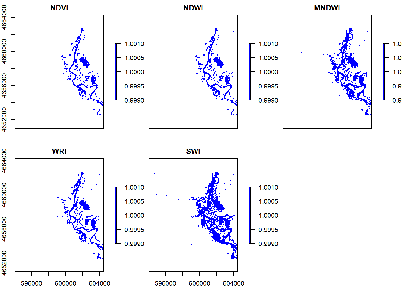
Image discussion:
The NDVI, NDWI, and WRI images are the most similar in that they show a lesser amount of flooded area compared to the SWI and MNDWI images. The SWI image highlights a wider flood area buffering the river and also picks up on other flooded areas outside of the rivers natural channel.
Binary flood masks vs. k-means cluster raster
| Image band | Area(m2) |
|---|---|
| NDVI | 5998500 |
| NDWI | 6489900 |
| MNDWI | 10742400 |
| WRI | 7621200 |
| SWI | 13680900 |
| k-means | 8194500 |